Post's a bit long this time, but juicy videos are at the end. Hang tough...
Last time I wrote about development of the dynamic model & kinematics using Simulink. I also explained the control strategy and showed some math associated with the phase plane diagram. Now we're ready to implement the controls in Simulink and run them with the HAPP dynamic model. Then we can tune the controller design before committing to hardware or software, and we can also investigate the effects of various issues like sampling rates of the onboard gyros and accelerometers. So here we go...
First, let's get a better picture of what we're trying to control. Imagine the HAPP as a large beach ball that we want to keep in a stable attitude with zero angular velocity. We have to stabilize around the three principal axes: X (pitch), Y (roll), and Z (yaw). The situation looks something like this:

To make the HAPP move with pure rotation around any one axis, we have to simultaneously fire two jets: One on each side of the HAPP. In the picture above, the two jets will cause rotation around the pitch axis when fired simultaneously.
Two more jets are needed to rotate in the opposite direction around the same axis. So to fully control the HAPP we need a total of 4 jets x 3 axes = 12 jets. However, jets will always fire in pairs, so we only need independent fire control for 6 pairs, a plus pair and a minus pair for each axis. The "fire plus" or "fire minus" decision for each axis will be implemented by one of three dedicated controllers.
Each controller needs to base its decision on where the HAPP is located in the phase plane for that axis relative to the switching curves, which were explained in the last post. The phase plane is defined by two state variables: Angular position and angular velocity. Fortunately we can easily read those from some MEMS gyros and accelerometers, similar to the ones you'd find in a modern mobile phone or tablet. I'll talk about the hardware in a later post - we're still doing everything in a simulation at this point.
The controllers don't look at the state variables per se. Rather, they look at an error signal which is defined as the difference between the current state variables and the desired state variables that are fed in to the autopilot. For example, if the desired attitude is "face due North", the attitude error would be the current heading - let's say 0.5 radians to the East - minus the heading for due North, which is 0 radians. The error is 0.5. Errors can be positive or negative. And don't forget that we can have errors for angular velocity as well; the target velocity is always 0 radians per second, unless of course we're purposely trying to place the HAPP into a slow spin (which might give some cool camera shots).
Now we feed our errors into the controllers and do the math. The controllers have to calculate where the HAPP is in the phase plane, decide which jets to fire so it moves toward the switching curves, reverse the jet fire at the curve, and maintain reverse fire until it reaches the origin (zero error signals). In summary, the controllers have to decide at any given time whether the HAPP is in a positive jet fire zone, a negative fire zone, or a coast zone (inside the deadband), and they have to issue the corresponding jet commands - for each set of jets on each axis. All of this decision making is an example of a control law.
As this is some fairly specialized logic for a control law, the easiest way to implement in Simulink is using an embedded MATLAB function. You can see the MATLAB code for one axis below. As a bonus, this code can be copied with minor modifications and put into the actual flight hardware someday. State variable errors go into the function, and jet fire commands come out. Shiny.
Here's a phase plane plot for one axis so you can see what the controller is thinking about. The thick red line is the HAPP's location in phase space (Quiz: Can you describe the attitude and rate errors that are present at the start of the video?). The controller fires jets one direction to reach the switching curve, drifts a bit through the deadband, then fires in the opposite direction to reach the origin.
Finally, because we will actually implement the control system in physical hardware some day, we must account for analog/digital conversions. Specifically, the MEMS gyros and accelerometers will send data to the flight computer at a certain sample rate (AD conversion). After the controllers issue fire commands, solenoid valves will open and gas will flow to the jets (DA conversion). Those AD/DA conversions have an effect on the performance of the control system, and we want to see it in the simulation. I haven't compensated for it yet in the controller design - it can wait until we get real hardware and see how it performs.
Putting it all together, we get a top-level view of the simulation that looks like this (yes I went through several versions before I got to v6 :-). I'm happy to share the project files if you're interested. The embedded MATLAB functions are hidden in a layer underneath the grey box labeled "Phase Plane Controller."
Long post - we're almost there. Just need to see it run! Well here you go... below are some traces from three of the scopes in the simulation. I adjusted the simulation so the video is showing the HAPP in real time - this is about how fast the HAPP will react to a good swift kick.
The top scope shows the attitude for each axis expressed in Euler angles (radians). In this example I gave the HAPP a pretty nasty "kick" and it's tumbling on all three axes. The controller and jets get everything stabilized after about 4 seconds.
The middle scope shows angular velocity in radians per second. You can see sharp changes as the jets fire. The angular velocity tends to change in a "V" pattern. The first side of the "V" is the controller driving the HAPP toward the switching curve on the phase plane. The second side is the controller driving it along the switching curve toward the origin (zero error). It tends to over-shoot due to rotation from the other axes "dragging" it away from the origin, and you can see all three axis traces repeatedly homing in with tighter and tighter errors.
The bottom scope shows the jet firing commands for each axis. The commands are either zero (coasting) or 2 (two jets firing to rotate in one direction around the axis - remember the beach ball). Things are a little messy because the HAPP is tumbling in three axes. If it was only spinning in one axis, you'd see those jets fire one direction (toward the switching curve) and then the other (toward the origin). Because it's spinning in other axes at the same time, it gets rotated away from this simple trajectory and has to continue compensating until everything settles down. Look at the rapid fire commands at about 4 seconds on the second axis... that would sound like a machine gun in real life. Can't wait to hear it!
Everything is looking good. Time to implement the controller in hardware & software. Next post....
Last time I wrote about development of the dynamic model & kinematics using Simulink. I also explained the control strategy and showed some math associated with the phase plane diagram. Now we're ready to implement the controls in Simulink and run them with the HAPP dynamic model. Then we can tune the controller design before committing to hardware or software, and we can also investigate the effects of various issues like sampling rates of the onboard gyros and accelerometers. So here we go...
First, let's get a better picture of what we're trying to control. Imagine the HAPP as a large beach ball that we want to keep in a stable attitude with zero angular velocity. We have to stabilize around the three principal axes: X (pitch), Y (roll), and Z (yaw). The situation looks something like this:

Two more jets are needed to rotate in the opposite direction around the same axis. So to fully control the HAPP we need a total of 4 jets x 3 axes = 12 jets. However, jets will always fire in pairs, so we only need independent fire control for 6 pairs, a plus pair and a minus pair for each axis. The "fire plus" or "fire minus" decision for each axis will be implemented by one of three dedicated controllers.
Each controller needs to base its decision on where the HAPP is located in the phase plane for that axis relative to the switching curves, which were explained in the last post. The phase plane is defined by two state variables: Angular position and angular velocity. Fortunately we can easily read those from some MEMS gyros and accelerometers, similar to the ones you'd find in a modern mobile phone or tablet. I'll talk about the hardware in a later post - we're still doing everything in a simulation at this point.
The controllers don't look at the state variables per se. Rather, they look at an error signal which is defined as the difference between the current state variables and the desired state variables that are fed in to the autopilot. For example, if the desired attitude is "face due North", the attitude error would be the current heading - let's say 0.5 radians to the East - minus the heading for due North, which is 0 radians. The error is 0.5. Errors can be positive or negative. And don't forget that we can have errors for angular velocity as well; the target velocity is always 0 radians per second, unless of course we're purposely trying to place the HAPP into a slow spin (which might give some cool camera shots).
Now we feed our errors into the controllers and do the math. The controllers have to calculate where the HAPP is in the phase plane, decide which jets to fire so it moves toward the switching curves, reverse the jet fire at the curve, and maintain reverse fire until it reaches the origin (zero error signals). In summary, the controllers have to decide at any given time whether the HAPP is in a positive jet fire zone, a negative fire zone, or a coast zone (inside the deadband), and they have to issue the corresponding jet commands - for each set of jets on each axis. All of this decision making is an example of a control law.
As this is some fairly specialized logic for a control law, the easiest way to implement in Simulink is using an embedded MATLAB function. You can see the MATLAB code for one axis below. As a bonus, this code can be copied with minor modifications and put into the actual flight hardware someday. State variable errors go into the function, and jet fire commands come out. Shiny.
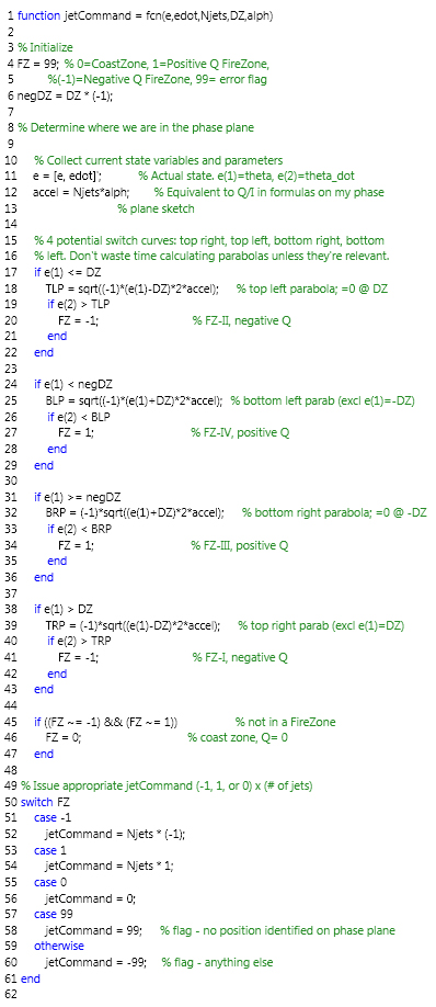 |
| Implementation of phase-plane control law for one axis. Inputs: State variables (e, edot), Jets per spin direction (N=2), Allowable deadzone (DZ), Jet moment divided by inertia tensor (alph). Inspired by Gran (2007) Ch. 9 but different logic flow. |
Here's a phase plane plot for one axis so you can see what the controller is thinking about. The thick red line is the HAPP's location in phase space (Quiz: Can you describe the attitude and rate errors that are present at the start of the video?). The controller fires jets one direction to reach the switching curve, drifts a bit through the deadband, then fires in the opposite direction to reach the origin.
Finally, because we will actually implement the control system in physical hardware some day, we must account for analog/digital conversions. Specifically, the MEMS gyros and accelerometers will send data to the flight computer at a certain sample rate (AD conversion). After the controllers issue fire commands, solenoid valves will open and gas will flow to the jets (DA conversion). Those AD/DA conversions have an effect on the performance of the control system, and we want to see it in the simulation. I haven't compensated for it yet in the controller design - it can wait until we get real hardware and see how it performs.
Putting it all together, we get a top-level view of the simulation that looks like this (yes I went through several versions before I got to v6 :-). I'm happy to share the project files if you're interested. The embedded MATLAB functions are hidden in a layer underneath the grey box labeled "Phase Plane Controller."
 |
| HAPP Flight Controller Simulink Model Blue = Constants; Grey = Controller & Dynamics; Yellow = Output; Orange = AD/DA; Red = Unused (translational dynamics) |
Long post - we're almost there. Just need to see it run! Well here you go... below are some traces from three of the scopes in the simulation. I adjusted the simulation so the video is showing the HAPP in real time - this is about how fast the HAPP will react to a good swift kick.
The top scope shows the attitude for each axis expressed in Euler angles (radians). In this example I gave the HAPP a pretty nasty "kick" and it's tumbling on all three axes. The controller and jets get everything stabilized after about 4 seconds.
The middle scope shows angular velocity in radians per second. You can see sharp changes as the jets fire. The angular velocity tends to change in a "V" pattern. The first side of the "V" is the controller driving the HAPP toward the switching curve on the phase plane. The second side is the controller driving it along the switching curve toward the origin (zero error). It tends to over-shoot due to rotation from the other axes "dragging" it away from the origin, and you can see all three axis traces repeatedly homing in with tighter and tighter errors.
The bottom scope shows the jet firing commands for each axis. The commands are either zero (coasting) or 2 (two jets firing to rotate in one direction around the axis - remember the beach ball). Things are a little messy because the HAPP is tumbling in three axes. If it was only spinning in one axis, you'd see those jets fire one direction (toward the switching curve) and then the other (toward the origin). Because it's spinning in other axes at the same time, it gets rotated away from this simple trajectory and has to continue compensating until everything settles down. Look at the rapid fire commands at about 4 seconds on the second axis... that would sound like a machine gun in real life. Can't wait to hear it!
No comments:
Post a Comment