Controls: Implementation (software and hardware)

It's finally time to go into hardware mode and start building stuff. Hoo-rah.

By this point in the project (not the blog) I was already a few months into it. Most of that time was spent reading the material in the bibliography and making sure I could work out the math by hand. I also spent a bit of time surfing the web and trying to learn from other people's efforts.

My general idea was to use an Arduino as the basis of the flight controller. I say "general idea" because prior to this project I had neither physically seen nor programmed an Arduino, Raspberry Pi, Intel Edison, or any other modern, programmable I/O board. I'd never even taken a course in C/C++. That means my starting point was the examples in my Arduino UNO Starter Kit. "This is an LED. Make the little LED go blinky-blink." I even took the 'duino, a breadboard, wiring, and some electronics components in my briefcase on an international business trip and fiddled in my hotel room at night while fighting jet lag. TSA never bothered to open my briefcase and look at the jumble of mysterious electronics :-/

For the actual flight hardware I chose an Arduino Mega 2560, not the UNO, because I thought I'd eventually use the extra pin-outs for other functions not related to the flight controller, such as environmental sensing and parachute deployment.

Onto the Mega went the Arduino 9 Axes Motion Shield. This is a complete inertial measurement unit (IMU) based on the Bosch BNO055 MEMS sensor package. It contains:

• A triaxial 14-bit accelerometer
• A triaxial 16-bit gyroscope
• A triaxial geomagenetic sensor
• A 32-bit microcontroller with software to fuse the data from these 3 sensors
• Capability to output quaternion data, Euler angles, angular acceleration, linear acceleration (which we won't use), gravity (how strong?), and heading (0-360 degrees on a compass).

It's sobering to compare the size of this IMU to the one on the Apollo spacecraft. The Bosch IMU measures only 5.2mm x 3.8mm x 1.1mm and is one of the tiny black bits on the Arduino shield in the right-hand photo below. It has no visible moving parts. Interestingly, the MEMS gyros are similar in structure and operation to the halteres of a fly, which rely on the Coriolis effect to encode the insect's body positions during flight.

Left: Old and busted.    Right: New hotness.

The 1960s Apollo IMU versus an Arduino Uno with 9 Axes Motion Shield.
The Bosch BNO055 IMU device is one of the tiny black bits on the shield.

It measures 5.2mm x 3.8mm x 1.1mm.

So down I go into my Mad Scientist Lair. A well-organized workshop is the foundation of success, right? At least that's how I justify to my wife why I spend the funds on kitting out the workshop. Thanks, Dear!

Espresso maker and liquor cabinet
are on the other side of that wall;
two additional and critical success factors.

First we check out the 9 Axes Motion Shield and confirm a few things. Is it communicating with the Arduino correctly? Does the data make sense - which way is up, what's a positive versus negative rotation, etc.? This picture summarizes the native output of Euler angles from the IMU:

BNO055 native output of attitude in radians

Here's a screen shot of the first data streaming from the shield, through the Arduino, and onto my PC through the serial monitor. Everything looks good.

Nothing like the smell of good data in the morning

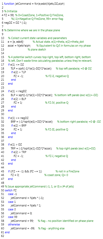
Next we tweak the embedded MATLAB function from the Simulink model so it will run on the Arduino. There were a few little tricks but basically it ported with minimal modifications. The main consideration is that we want the code to loop as fast as possible, as this will give the highest refresh rate for the sensor readings. The code imposes some simple logic checks and only calculates the relevant portion of the switching curves to determine which fire zone or coast zone it inhabits on the phase plane. I'm happy to share the code with anyone interested, although it's specific to the Bosch IMU and may need to be tweaked for your sensor, particularly for the rotation sequence of Euler angles.

Even with live output to the serial monitor, the final version of the code gives a refresh time of about 7 milliseconds, which is almost 150 Hz. The Apollo Lunar Module's flight computer had a refresh rate of 100 ms so we're already doing better than the 1960s. In addition, many solenoid valves I've seen have an activation time around 20 ms and an on/off cycle even slower, so the HAPP software is already outrunning the hardware and may have to be "slowed down" anyway.

The last step is to get the Adruino - now programmed as the flight controller - to turn power relays on and off according to the jet firing commands. Recall that we need 6 independent fire control circuits, each of which will fire two jets simultaneously to apply moment around a particular axis. The relays will switch power to the gas solenoid valves, which in turn allow compressed gas to flow to the jet nozzles. I haven't specced out the valves yet, but some quick research showed that the valves might require up to 24 Volts DC and perhaps 0.2 Amps.

For now I'm using this 8-channel electromagnetic relay. For the flight hardware I'll replace it with solid-state relays or MOSFETs. Either one would have a faster response time than the electromagnetic relays, on the order of milliseconds or less. That will help with performance of the flight controller.

Enough talk - let's see it run. In the following video, six relays are labeled by jet command: Yaw +, Yaw -, etc. You can see and hear the relays turning on and off as the flight controller is rotated in space relative to the target setting of [0, 0, 0] attitude and [0, 0, 0] angular velocity. When the HAPP is complete, these relays will trigger solenoid valves and the jets will fire. The flight controller has a deadband of 7 degrees so I have to rotate it quite a bit to trigger the relays. Later we will reduce the deadband to give tighter performance and more highly stabilized video.

That's about it for the brains of the HAPP, although later we'll be adding additional hardware for environmental sensing, system monitoring (gas tank pressure, etc.), and some other tasks. Now it's time to figure out how to make the jets. Get ready for some thermodynamics...

Controls: Simulation results

Post's a bit long this time, but juicy videos are at the end. Hang tough...

Last time I wrote about development of the dynamic model & kinematics using Simulink. I also explained the control strategy and showed some math associated with the phase plane diagram. Now we're ready to implement the controls in Simulink and run them with the HAPP dynamic model. Then we can tune the controller design before committing to hardware or software, and we can also investigate the effects of various issues like sampling rates of the onboard gyros and accelerometers. So here we go...

First, let's get a better picture of what we're trying to control. Imagine the HAPP as a large beach ball that we want to keep in a stable attitude with zero angular velocity. We have to stabilize around the three principal axes: X (pitch), Y (roll), and Z (yaw). The situation looks something like this:

To make the HAPP move with pure rotation around any one axis, we have to simultaneously fire two jets: One on each side of the HAPP. In the picture above, the two jets will cause rotation around the pitch axis when fired simultaneously.

Two more jets are needed to rotate in the opposite direction around the same axis. So to fully control the HAPP we need a total of 4 jets x 3 axes = 12 jets. However, jets will always fire in pairs, so we only need independent fire control for 6 pairs, a plus pair and a minus pair for each axis. The "fire plus" or "fire minus" decision for each axis will be implemented by one of three dedicated controllers.

Each controller needs to base its decision on where the HAPP is located in the phase plane for that axis relative to the switching curves, which were explained in the last post. The phase plane is defined by two state variables: Angular position and angular velocity. Fortunately we can easily read those from some MEMS gyros and accelerometers, similar to the ones you'd find in a modern mobile phone or tablet. I'll talk about the hardware in a later post - we're still doing everything in a simulation at this point.

The controllers don't look at the state variables per se. Rather, they look at an error signal which is defined as the difference between the current state variables and the desired state variables that are fed in to the autopilot. For example, if the desired attitude is "face due North", the attitude error would be the current heading - let's say 0.5 radians to the East - minus the heading for due North, which is 0 radians. The error is 0.5. Errors can be positive or negative. And don't forget that we can have errors for angular velocity as well; the target velocity is always 0 radians per second, unless of course we're purposely trying to place the HAPP into a slow spin (which might give some cool camera shots).

Now we feed our errors into the controllers and do the math. The controllers have to calculate where the HAPP is in the phase plane, decide which jets to fire so it moves toward the switching curves, reverse the jet fire at the curve, and maintain reverse fire until it reaches the origin (zero error signals). In summary, the controllers have to decide at any given time whether the HAPP is in a positive jet fire zone, a negative fire zone, or a coast zone (inside the deadband), and they have to issue the corresponding jet commands - for each set of jets on each axis. All of this decision making is an example of a control law.

As this is some fairly specialized logic for a control law, the easiest way to implement in Simulink is using an embedded MATLAB function. You can see the MATLAB code for one axis below. As a bonus, this code can be copied with minor modifications and put into the actual flight hardware someday. State variable errors go into the function, and jet fire commands come out. Shiny.

Implementation of phase-plane control law for one axis.
Inputs: State variables (e, edot),
Jets per spin direction (N=2),
Allowable deadzone (DZ),
Jet moment divided by inertia tensor (alph).
Inspired by Gran (2007) Ch. 9 but different logic flow.

Here's a phase plane plot for one axis so you can see what the controller is thinking about. The thick red line is the HAPP's location in phase space (Quiz: Can you describe the attitude and rate errors that are present at the start of the video?). The controller fires jets one direction to reach the switching curve, drifts a bit through the deadband, then fires in the opposite direction to reach the origin.

Finally, because we will actually implement the control system in physical hardware some day, we must account for analog/digital conversions. Specifically, the MEMS gyros and accelerometers will send data to the flight computer at a certain sample rate (AD conversion). After the controllers issue fire commands, solenoid valves will open and gas will flow to the jets (DA conversion). Those AD/DA conversions have an effect on the performance of the control system, and we want to see it in the simulation. I haven't compensated for it yet in the controller design - it can wait until we get real hardware and see how it performs.

Putting it all together, we get a top-level view of the simulation that looks like this (yes I went through several versions before I got to v6 :-). I'm happy to share the project files if you're interested. The embedded MATLAB functions are hidden in a layer underneath the grey box labeled "Phase Plane Controller."

HAPP Flight Controller Simulink Model
Blue = Constants;
Grey = Controller & Dynamics;
Yellow = Output;
Orange = AD/DA;
Red = Unused (translational dynamics)

Long post - we're almost there. Just need to see it run! Well here you go... below are some traces from three of the scopes in the simulation. I adjusted the simulation so the video is showing the HAPP in real time - this is about how fast the HAPP will react to a good swift kick.

The top scope shows the attitude for each axis expressed in Euler angles (radians). In this example I gave the HAPP a pretty nasty "kick" and it's tumbling on all three axes. The controller and jets get everything stabilized after about 4 seconds.

The middle scope shows angular velocity in radians per second. You can see sharp changes as the jets fire. The angular velocity tends to change in a "V" pattern. The first side of the "V" is the controller driving the HAPP toward the switching curve on the phase plane. The second side is the controller driving it along the switching curve toward the origin (zero error). It tends to over-shoot due to rotation from the other axes "dragging" it away from the origin, and you can see all three axis traces repeatedly homing in with tighter and tighter errors.

The bottom scope shows the jet firing commands for each axis. The commands are either zero (coasting) or 2 (two jets firing to rotate in one direction around the axis - remember the beach ball). Things are a little messy because the HAPP is tumbling in three axes. If it was only spinning in one axis, you'd see those jets fire one direction (toward the switching curve) and then the other (toward the origin). Because it's spinning in other axes at the same time, it gets rotated away from this simple trajectory and has to continue compensating until everything settles down. Look at the rapid fire commands at about 4 seconds on the second axis... that would sound like a machine gun in real life. Can't wait to hear it!

Everything is looking good. Time to implement the controller in hardware & software. Next post....

Controls: Strategy and control law

I started this blog yesterday, but in truth I've been working on the HAPP project for a few months and I've made some real progress. I'm just catching up with the blogging :-)

So I'll start off where I began the real work: The control system. Before thinking about hardware and software, I figured I'd need a firm grasp on the controls theory needed to fly the HAPP autonomously. It would be nice to use an existing open-source flight controller like this, but as I'm going to use something like 12 gas jets instead of 4 propellers on a drone, I assumed that rolling my own controller would not be much worse than trying to modify an existing one. Plus, I'm just a roll-your-own kind of guy...

For those who care, I've posted a short bibliography here that contains some books and articles that I found particularly useful. It was a great refresher course as I hadn't really thought deeply about controls theory since grad school back in the early 1990s. Even then I never had the chance to study spacecraft dynamics and control, so some topics were new to me. Real controls gurus may roll their eyes at the material in this post, but it was my first time through some of it and I had fun learning. So there!

First up were dynamics and kinematics. For aircraft and spacecraft, we typically want to model both the translational motion (trajectory) and the orientation (attitude), and we have to keep track of our frame of reference (kinematics) - relative to the craft, to the ground, or to elsewhere. For the HAPP, I really don't care where it comes down, even if it blows 50 miles away from the launch site. In addition, it would take an entirely different strategy to actively "fly" it back home, and then we'd be talking about designing some sort of high altitude glider like this (nice job guys!). For those reasons I chose to neglect translational motion and simply focus on getting a nice, stable attitude for the cameras. Let the winds carry it where they may... we'll find it with GPS tracking.

Knowing that I'd eventually want to implement the control system in a simulation before investing time to create real hardware and software, I modeled the rotational dynamics and kinematics in Simulink. I had to purchase the MATLAB/Simulink suite as I've not needed them since grad school. Needless to say, they've evolved a bit since the early 90s... a couple of all-nighters doing tutorials over the weekend and I was ready to rock. This book was a huge help. It's the best reference I've seen for getting up to speed quickly in Simulink.

I spent a few hours implementing the model based on the outline in this paper. The model utilizes quaternion-based kinematics, which are a nice way to describe rotations in three axes. Quaternions are computationally friendly compared with the alternatives like Euler angles and Direction Cosine Matrices (which is why, as I learned, that quaternion-based models are also used for 3D graphics).

Once everything was running smoothly, I discovered that for $45 I can purchase an aerospace blockset for Simulink that has the same math conveniently available in a pick-and-place modeling block. So we'll just write my efforts off as an edifying exercise and a nice double-check on the maths :-/

Top layer of the quaternion-based dynamics model. Maths r fun!

With the model in place, what about the controls strategy? The general class of problem we're trying to solve is called a two-point boundary value, minimal time, optimal control problem. That's a fancy-pants way of saying that the HAPP is in one position, possibly spinning with some angular velocity, and we want to return it to a target attitude with zero spin. Furthermore, we want to do it as quickly as possible. In other words, we want it to stabilize its position and spin so we get nice clean video.

It turns out the optimal control law for this class of problem is known as a bang-bang controller. It starts by turning on the jets in one direction to counteract the spin and begin moving the HAPP into the desired attitude. Then, at a certain point, the jets fire in the opposite direction to slow it down and "land" it in the target attitude with zero spin.

To use a car analogy, it's similar to the following problem: How do you get a car from point A to point B in the least amount of time, with the condition that it must stop at point B without over-shooting? Answer: Stomp on the gas pedal all the way (bang!), accelerating as fast as possible. Then, at a certain point, stomp on the brakes as hard as you can (bang!). The trick is to determine that certain point.

Propeller-driven drones typically utilize a PID controller which can vary the speed of each propeller within some range from zero to max. That's a different type of controller - it's not all-or-nothing; it's not bang-bang. For cold-gas jets, typically they are turned on and off with solenoid valves, and therefore are either firing at 100% or not firing at all. There are proportional valves available but we don't need them - we actually want the simple on/off solenoids to implement the bang-bang controller. This is exactly the type of controller used in the autopilot for NASA's Apollo Lunar Lander back in the 1960s (try your hand at landing the Eagle manually here!).

That "certain point" is called a switching curve. Why is it a curve? Well, start by making a graph with the rotational position on the x-axis, and the rotational or angular velocity on the y-axis. This is a phase-plane diagram. Given the physical properties of the HAPP (specifically the inertia tensor and the moment produced by the jets), it can only move in certain trajectories on the phase plane when we apply a moment by firing the jets. We want to drive the HAPP to the origin of this graph - zero angular velocity, and zero angular position versus the target. It turns out there is a parabolic curve through the origin that the HAPP can "follow" back to zero by firing its jets continuously. Being on this curve is like being in the stomp-the-brakes phase from the car analogy. But to reach this curve and stomp the brakes, we first have to fire jets in the direction opposite from the braking one. Putting it all together, we fire jets in one direction until we reach the switching curve, and then we switch and fire jets in the opposite direction until we reach zero spin/zero position error.

After some math and a little sketching, I generated the switching curves and was ready to build the controller in Simulink. You might notice two sets of curves in the picture: red and green. What's that all about? The two switching curves are separated by a deadband to prevent an over-active controller that essentially fires jets almost all the time. I'll leave it to you to read up on that topic.

Next time: Implementing the controller in Simulink...

Switching curve plots and formulas. X-axis = attitude; Y-axis = angular velocity;
FZ = fire zone; CZ = coast zone; +Q = positive jets; -Q = negative jets.
The quadrants I-IV represent conditions to check in the controls software.

First post!

All your high altitude base are belong to us...

Well I've been thinking about this insane project for several months now, and as of Spring 2016 I finally decided to invest the time and money to see if I can pull it off.

My motivation is simple: I like photography, especially the more technical stuff, and aesthetically speaking I like low-light images of cities, mountains, and sky. I want to get some pristine images and video from the edge of space, or as close as I can get. Given the recent emergence of VR video, it might even be fun to capture 360-degree HD video and "take a look around."

The interwebs are full of people who have sent small cameras up on weather balloons and gotten some images, such as here and here and here. Occasionally they get lucky and are able to pull a decent still photo or perhaps a few seconds of usable video. But the majority of video clips are nausea-inducing due to their lack of stabilization. At lower altitudes the winds wreak havoc. At apogee the bursting of the weather balloon sets the camera tumbling. Anyone who even attempts such a feat has earned some serious geek cred, but there has to be a better way...

If there was any significant atmosphere at 30Km altitude the camera could be stabilized by aerodynamic forces, perhaps like a quadcopter drone with propellers. Alas, the air at 30Km is as rare as hen's teeth, and to actively stabilize a camera platform you'd have to employ one of the strategies used by spacecraft, such as momentum wheels or reaction control jets.

After seeing this project by some students at Portland State (nice job guys!) and boning up on the engineering behind various spacecraft systems, I concluded that a cold gas reaction control system or RCS was probably the best candidate in terms of minimal mass and maximum simplicity. Of course, simplicity is a relative term...

In the many months until launching the HAPP and getting some nice footage to share on this blog, I'll periodically post some of my ground-based work just to keep the creative juices flowing. Many of the pics are also available on my general photography site here.

For now, enjoy some summer star trails over Traverse City, Michigan...

(c) Christopher Couch 2015